How to Use SUMIFS with Criteria Lists, Summarizing Sales

With one exception, SUMIFS is a very powerful function. And it’s very fast.

To understand the one exception, suppose you have a table of sales by product by date…as shown in Example 1, below. It’s easy to use a SUMIFS function to return the sales for one of those products.

Here’s the syntax for the SUMIFS function:

=SUMIFS(sum_range,  criteria_range,criteria, …)

And this formula, shown in the Example 1 figure below, returns total sales for the product name entered in cell G7:

H7:   =SUMIFS(Amt, Prod,G7)

That is, in this formula, SUMIFS returns the sum of all values in the Amt column for which the corresponding item in the Prod column matches the single item in cell G7.

This also is true of other “S” functions like AVERAGEIFS, COUNTIFS, MAXIFS, and MINIFS. We can use these functions to summarize information about the Hats product or the Coats product; but we can’t use one formula to summarize the of sales for Hats and Coats…

…Or can we?

In the following examples I’ll show you how to set up SUMIFS and COUNTIFS functions so they can summarize your data from lists of criteria, and I’ll give you some ideas about how you might use this new capability.

Example 1: Return Data from a Sales Database

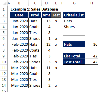Here, we have a simple database of sales by month by product.

What we want to do is to be able to enter a variable number of product names in the Criteria List and see the total of all sales for those products in the List Total cell.

That is, we want to use one SUMIFS formula to return the total for not just one product—as shown in cell H7—but for any number of products we want to add to our list.

Rather than telling you what to do, let me tell you how I figured out how to do it…

I started with this formula:

H7:   =SUMIFS(Amt,  Prod,G7)

Here, of course, I knew that cell G7 is the criteria argument for the first (and only) criteria range for this formula. And Excel is expecting a single value for that criteria.

But I also knew that if we specify a range of cells for an argument that asks for only one cell, and then we array-enter the formula, Excel will return an array of results, one for each item in the list.

So when I array-entered…

H7:   =SUMIFS(Amt,  Prod,CriteriaList)

…that is, when I pressed Ctrl + Shift + Enter after I typed in the formula, I got an answer of 36…which was the same result I had in cell H7 originally. I was slightly confused at first, because it looked like nothing much had happened. But then I clicked in the formula bar and pressed the F9 key…

…where I saw this result:

={36;6;0}

Now everything made sense. Excel calculated the sum for each item in the Criteria List, but returned only the first item in the array…which was the value 36.

Therefore, because I wanted the sum of all those items, I array-entered this formula…

H7:   =SUM(SUMIFS(Amt,  Prod,CriteriaList))

…and got the value of 42, which is the value I was looking for.

However, working with array formulas is kind of a pain. So, I wondered if I could set this up so that I wouldn’t have to enter my formula as an array.

I knew that the SUMPRODUCT function treats its arguments as an array, and you don’t have to array-enter it. So I entered this formula normally:

H7:   =SUMPRODUCT(SUMIFS(Amt,  Prod,CriteriaList))

And sure enough, I got 42 again.

Outstanding!

Then I moved the formulas around a little so that cell H7 held my original version again, and I put my final version here:

H9:   =SUMPRODUCT(SUMIFS(Amt,  Prod,CriteriaList))

But now, I wondered, what if I had thousands of items in my table. How could I ensure that I had the correct result in cell H9? That’s why I set up the Test column.

Here’s the formula for the first cell in the Test column…

E3:   =IFERROR(IF(MATCH(C3,CriteriaList,0),”x”),””)

This formula tells Excel to use an exact match (because its third argument is zero) to search the CriteriaList column for the value in cell C3. Because I didn’t care what the MATCH value was, I set it up just to return “x” if MATCH returns any numeric value at all.

This formula uses two shortcuts that I should explain…

First, I didn’t need to include the test
MATCH(whatever)<>0 because the IF function treats non-zero values as TRUE, and it treats ZERO values as FALSE. In other words, this formula =IF(3,”x”) returns “x”, because the IF function treats 3 as TRUE.

Second, I didn’t need to include the third argument in the IF function, because IF automatically returns FALSE if the first argument isn’t TRUE. That is, =IF(0,”x”) returns FALSE.

However, remember that MATCH returns #N/A—not zero—if no value is found. And that means we’d never see the IF function’s FALSE value in any case. Instead, we’d get that an #N/A value as an error. Therefore, I enclosed the formula in an IFERROR function so it would return a null string if the IF function returns an error value—the #N/A in this case.

By the way, I also could have used…

E3:   =IF(ISNA(MATCH(C3,CriteriaList,0)),””,”x”)

…which probably would have been easier to understand, but I thought of the other method first.

In any case, after I entered the formula, I copied it down the Test column, giving me the results shown in column E above. Then, to test my result, I entered this formula…

H10:   =SUMIFS(Amt,  Test,”x”)

…which gave me the same result as in cell H9.

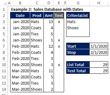
Example 2: Return Sales Totals with Dates

I’ll try to make this example fast.

Often, when we have a table of data that includes dates, we’ll want to return subtotals for a range of dates.

So this example adds to the previous example the ability to specify dates.

Because I was doing this in a hurry, and because I wanted to keep the example figures as narrow as possible, I called the first date Start and the second date Stop.

In real life, of course I would have used more descriptive titles. But in any case, here’s the formula that uses those date values:

H10:   =SUMPRODUCT(SUMIFS(Amt,   Prod,CriteriaList,   Date,”>=”&Start,
Date,”<=”&Stop))

Notice two things about this formula…

First, there are several spaces between “Amt,” and “Prod”, and between each remaining pair of arguments after that. In other words, I set up the SETIFS part of the formula something like this:

=SUMIFS(sum_range,   criteria_range,criteria   criteria_range,criteria  criteria_range,criteria,    …)

When you add spaces between arguments like that, Excel ignores the spaces. But I find them very useful for visually separating each set of criteria range and its criteria.

Second, notice that I use Date as the criteria range twice. That’s no problem at all. I tested it the first time to look for all dates greater than or equal to the Start date, and the second time to filter all dates that are less than or equal to the Stop date. In combination, those two tests identify all dates between the Start and Stop dates, inclusive.

Example 3: Return Sales by Region When Region Isn’t Listed

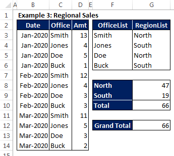In this example, I show a table of sales by Office, which have the unusual names of Smith, Jones, Doe, and Buck.

What we want to do is to summarize those sales by Region even though the table doesn’t include a Region column.

When I had to report summaries like this before I figured out the formulas I’m showing you, I’d have to add a Region column to my table, use INDEX-MATCH to return the correct region for each Office, and then write my SUMIFS formulas to filter on that new Region column.

But when you use a list of criteria with your SUMIFS formulas, that extra effort isn’t needed. Here’s the formula for the cell shown:

G8:   =SUMPRODUCT(SUMIFS(Amt,  Office,OfficeList)*(Region=F8))

Here, the four-cell SUMIFS array returns a total for each Office in the OfficeList, no matter which Region it’s in. But then, the formula multiplies those results by (RegionList=F8), which acts as a four-cell array in this SUMPRODUCT formula, because Region also is a list.

(Notice that I multiplied two four-cell arrays. You can multiply arrays like this only when each array has the same dimension.)

Because cell F8 contains “North”, the (Region=F8) array resolves to the array {TRUE;FALSE;TRUE;FALSE} when it’s used in the formula in cell G8. And then, when the formula multiplies that array of TRUE and FALSE values, the TRUE values are interpreted as 1 and FALSE vales as zero.

As a consequence of this multiplication, cell G8 returns the sum of only the North Region’s values, because multiplying by the FALSE values turns the other sums to zero.

Similarly, for the South Region, we have…

G9:   =SUMPRODUCT(SUMIFS(Amt,Office,OfficeList)*(Region=F9))

…and the formula returns the total of the SUMIFS results only for the Offices belonging to the South region.

And finally, the total of those two results shown in cell G10 matches the simple calculation in this cell:

G12:   =SUM(Amt)

In How to Create Summarized Financial Statements with SUMIFS Criteria Lists, I continue these examples by showing you how to find totals in tables of income-statement data, even when the signs of the numbers normally would make that difficult to do.

And finally, in Advanced SUMIFS Calculations with Criteria Lists, I show you a variety of short examples to finish off this series. For example, if you have a table that shows only sales by product, I’ll show you how one formula can return the gross profits for all those sales.